Have you gone in for your annual fiscal yet?
Even as US citizens do exactly that while filing their tax returns, US states and the companies they covet are undergoing scrutiny of their own fiscal health. Their probing and poking, however, is a constant, rather than annual, affair.
New reports and online resources from the Mercatus Center at George Mason University and the Pew Charitable Trusts shine welcome light on each state’s strengths and weaknesses.
From the Mercatus Center at George Mason University comes “State Fiscal Condition: Ranking the 50 States,” a white paper authored by Dr. Sarah Arnett, who wrote her 2011 PhD dissertation about how to measure fiscal stress in the U.S. states along with how states respond to different levels of fiscal stress. She is currently an analyst at the federal Government Accountability Office (GAO).
Her study uses 2012 data from states’ comprehensive annual financial reports (CAFRs) to rank each state based on four solvency measures, based on a model promulgated by the International City/County Management Association (ICMA). Arnett then takes those results and compiles a composite index from those rankings, depicted in this map:
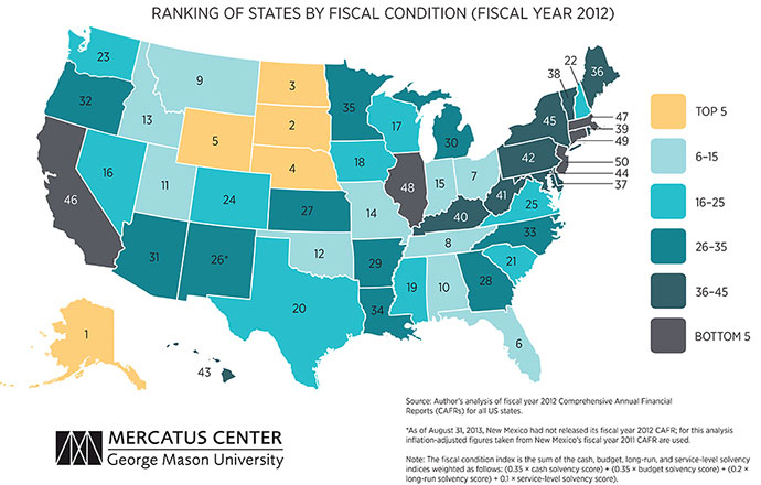
“The five states with the highest-ranked overall fiscal condition are Alaska, South Dakota, North Dakota, Nebraska and Wyoming,” reports Arnett. “The five states with the lowest-ranked fiscal condition are New Jersey, Connecticut, Illinois, Massachusetts, and California. The top five states all had a surplus in fiscal year 2012 as measured by an increase in net assets, but there are differences in their underlying strengths. I find that the states with the worst fiscal condition have had years of poor financial management across the different dimensions of fiscal condition.”
The results of Arnett’s analysis closely correspond to fiscal health analysis from the Pew Center on the States, which released its “Fiscal 50” online tool in November to examine the various risk and volatility factors that any site evaluator might wish to study before planting a company’s flag in a given territory. Pew’s map showing the states’ relative increases or decreases in spending resonates with Arnett’s findings.
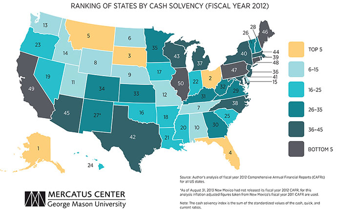
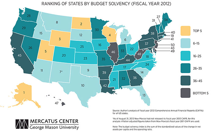
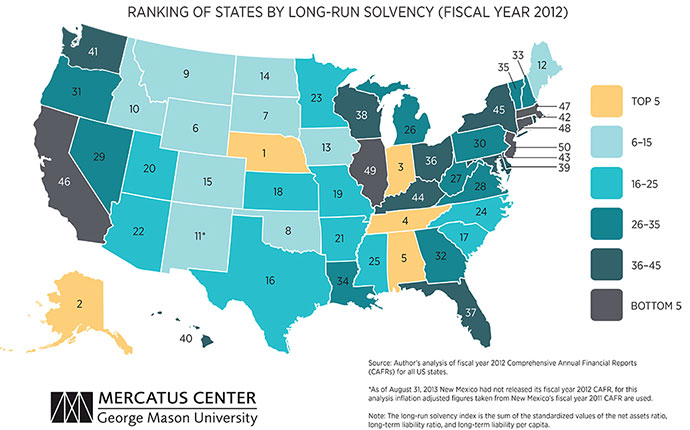
Here are the definitions of each of the four categories in Arnett’s analysis, accompanied by highlights of the report’s findings and maps depicting the rankings within each:
A state’s cash solvency reflects the cash it can easily access to pay its bills in the near term, or the state government’s liquidity. “Alaska maintains a high cash balance to accommodate the quarterly volatility of its main revenue source, petroleum tax revenue,” the report states. “On the other end of the rankings, despite improvements in its economic conditions, California still ranks near the bottom in cash solvency.”
A state’s budget solvency is its ability to create enough revenue to cover its expenditures over a fiscal year. “Two of the top-ranked states, Alaska and North Dakota, have benefited from increased revenues due to natural resource extraction and higher oil prices … New Jersey was ranked at the bottom in budget solvency, largely due to a decrease in net assets of $6.4 billion.”
Long-run solvency measures each state’s ability to cover all of its costs with incoming revenue, including long-term obligations such as guaranteed pension benefits and replacing infrastructure. Relative to the other measures, long-run solvency is less sensitive to economic trends. Nebraska is No. 1, says the report, in part because it’s constitutionally prohibited from incurring debt.
“As such, the long-term liabilities reflected in Nebraska’s long-run solvency score are mainly due to claims payable for worker’s compensation, Medicaid claims, and other employee-related items,” says the report. With no significant bond debt, Nebraska has a much lower long-term liability per capita and a much lower long-term liability ratio than most other states.
“At the bottom of the rankings are New Jersey and Illinois. New Jersey faces long-run solvency problems due in part to nearly 15 years of underfunding its state and local pensions. It has an estimated unfunded pension liability of around $25.6 billion as well as $59.3 billion in unfunded liabilities for the health benefits of retired teachers, police, firefighters, and other government workers (State Budget Crisis Task Force 2012). Illinois has also underfunded its public pensions, resulting in an estimated state retirement system combined unfunded liability of $96.8 billion as of 2012 (Illinois Commission on Government Forecasting and Accountability 2013). To cover the costs of its pension obligations, Illinois has also sold bonds to cover its annual contributions — 60 percent of Illinois’s total outstanding debt is in pension bonds (State Budget Crisis Task Force 2012). In essence, Illinois is using long-term debt instruments to meet current year pension obligations.”
Service-level solvency reflects whether state governments have the resources to provide their residents with an adequate level of services.
“Comparing the top-ranked Nevada to the bottom-ranked Alaska provides some insight into the difficulties in interpreting this solvency index,” writes Arnett. “Nevada has relatively low values for taxes per capita ($1,492), revenues per capita ($3,393), and expenses per capita ($3,266) when compared to the 50-state averages …. As applied to service-level solvency, these low values are interpreted as allowing room for future growth in taxes or services as needed — meaning Nevada has a better expected ability to pay for services. Nevada’s reliance on sales and gaming taxes and not on a state income tax is seen as evidence of state flexibility to add tax bases and revenues as needed to accommodate potential future demand.
“Alaska, by contrast, has relatively high values for taxes per capita ($9,825), revenues per capita ($19,137), and expenses per capita ($13,873). These per capita figures conceal the fact that Alaska has neither a state personal income tax nor a sales tax. Indeed, the lack of these two taxes suggests that Alaska has quite a bit of flexibility in increasing taxes, if needed.”
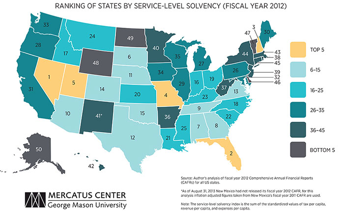
Arnett notes at the outset that fiscal health is difficult to measure, with the service-level category being the most difficult, and therefore the least weighted in the composite score. Giving equal weight to all still resulted in Alaska at the top and New Jersey at the bottom, with Wisconsin (11 spots) and North Dakota (12 spots) each moving down due to low service-level scores.
“The level and quality of services a government should provide are highly variable, depending on political and taxpayer preferences,” she writes. “Higher taxes and revenue per capita suggest a higher tax and revenue burden on state residents. Higher taxes per capita suggest that the government is already providing an expensive level of services; as such, its ability to provide more services due to a change in economic condition or demographics is more difficult because there is less room for tax increases. Similarly, a state with high expenses per capita may not be allocating resources in the most efficient or productive manner, leaving it vulnerable if service demands increase. However, low levels of taxes or revenues per capita may be due to a recession or an inefficient tax regime, not a system with room to adapt to new service demands.”
Among her observations is this statement (bibliographical references deleted), which encapsulates some of the gray area that location decision-makers traverse every day in evaluating territory-based policy risk:
“Time is the main source of imprecision found in the long-run and service-level solvency indices … As Jacob and Hendrick (2013) discuss, long-run and service-level solvency depend on how governments will act in the future, which is unknown at the current time. Service-level solvency may depend on a decision a state makes about its tax structure (tax rates or the type of taxes collected) or the level and cost of services provided (service needs and political/resident demand for services).”
Arnett notes that credit ratings such as Standard & Poor’s are strongly correlated to her fiscal condition index, albeit focused on a much broader range of factors including demographics and fiscal structure.
Smoothing Out the Bumps
Nov. 2013 analysis by Pew’s Jeff Chapman and Julie Srey, part of a comprehensive suite of tools and data called “Fiscal 50: State Trends and Analysis,” noted that the employment rate in pre-recession calendar year 2007 among people ages 25 to 54 was around 80 percent, and in the fiscal year ending June 2013 was around 76 percent. Thus tax revenue, among other factors, has declined. “The largest decline in the employment rate was in Nevada, where 73.8 percent of prime-age workers had jobs in fiscal 2013 — 8.3 percentage points lower than in 2007,” they observed. “Among the least affected were Nebraska and Vermont, which saw the smallest observable changes from their current employment rates of 84.9 and 82.6 percent, respectively.”
Another Pew report, released this week, is titled Managing Uncertainty: How State Budgeting Can Smooth Revenue Volatility, is the first in a series designed to provide strategies to policymakers to improve long-term state fiscal health, and examines patterns of state economic and revenue fluctuation over the past 20 years. The analysis reveals wide variation in the degree to which revenues change over time and identifies state economic characteristics and tax systems as factors influencing volatility. Pew’s research also finds that, on average, state revenues vary more dramatically than do their underlying economies.
The study, based on data from two full economic cycles from 1990 to 2012, identifies three practices that can help policymakers (many of whom are in session as you read this) chart a clearer direction through the fiscal uncertainty caused by unforeseeable changes in revenue:
“States should study the causes of volatility in their economies and their impact over time. These studies should be released on a regular schedule, examine which areas of the tax system and the economy are volatile and why, and include recommendations for fiscal policies to manage uncertainty.”
“States should revise revenue forecasts as close to the final passage of the state budget as possible and plan for possible shortfalls or surpluses. Although revenues can be inherently difficult to predict, states can develop their projections as close to key budget decisions as possible and have processes in place to better respond to forecasting errors.”
“States should develop or refine budget policies that run counter to economic cycles and save money during growth periods for use in down times. States can create reserves, or rainy day funds, so that saving money during good times is a consistent, predictable practice based on specific drivers of revenue volatility.”

